As a data backup and recovery company, it’s no great surprise that over 50% of Rewind’s AWS spend goes to storage. Specifically, S3 storage.
We recently embarked on a project to see if we could lower our overall AWS spend. We are always optimizing for cost across various AWS services by leveraging savings plans and reserved instances, using AWS Graviton processors where possible, and employing various service-specific optimizations. But with storage being the main cost center, we set out to look for efficiencies.
At the start of this project, we were using over 10 petabytes (PB) of storage, tiered across multiple storage classes to optimize overall storage costs. With a closer look at the data in S3, we found significant duplication. That is, data that all had the same hash within S3. In fact, it was 60 billion objects consuming 3.5 PB of storage!
This post will cover why we had so much duplicate data and then go into some detail about how we were able to remove it to realize major storage savings without any sacrifice. As we have discovered many times over the years, dealing with small amounts of data is trivial—but dealing with hundreds of billions of objects in S3 makes even simple tasks like deleting data an interesting technical challenge without breaking the bank. We also had to do all this while not affecting the live, running system which is performing tens of thousands of backups daily.
Backups and duplicate data
Rewind backs up multiple SaaS platforms via the use of REST or GraphQL public APIs. There’s a lot of complexity here (and complexity only increases when restoring the data) but to simplify the process: During a backup, Rewind asks: “what has changed since the last time we backed up a particular item?” Most of the platforms we back up have what we call “nested items” where a particular item is a child of a parent item and is backed up along with the parent.
In the case of Rewind for Shopify, one of the key items we back up is products (makes sense for an eCommerce store!) and nested under products are product images. When we detected a change in a product—for example, an inventory level change—we would also back up the product AND the product images even if they had not changed. This results in a significant number of image files that are essentially duplicated as they have not changed. How significant was this? We estimated that somewhere around 80% of the storage consumed by Shopify backups was product images and of these, 80% were duplicates. A very high percentage indeed.
We attacked this problem from two sides. The engineering team took advantage of a newer item in Shopify called Product Media. This allowed us to back up images independent of the product. In other words, to only back up product specific changes rather than having these images duplicated by always ‘nesting’ them under a new version of a product.
This solved the problem going forward but we were still storing 10 years’ worth of backup data and a lot of duplicate images among it.
Dealing with the existing data is the focus of this article. We had to characterize the problem: how much space did these duplicates consume? How many objects was it? How much could we potentially save if we removed these? And ultimately, we had to determine if it was even worth spending any time on this.
Spoiler alert: it was.
Data analysis
We used S3 Inventory reports to analyze where the duplicates resided and to give us an estimate into the amount of data we were looking at in terms of storage use and number of objects. Doing this was reasonably straightforward:
- Enable S3 inventory reports on the S3 bucket(s). As an example, we used the ORC format and made sure we exported the etag in the inventory data.
- Create an Athena table to be able to query the inventory reports.
One problem area we found here was that the inventory reports were so big, Athena had a problem querying them. We used partitioning and bucketing to reduce the data sets we had to query with Athena.
A base S3 inventory table in Athena looks like this:
CREATE EXTERNAL TABLE `inventory_weekly_with_etag`( `bucket` string, `key` string, `version_id` string, `is_latest` boolean,
`is_delete_marker` boolean, `size` bigint, `last_modified_date` timestamp, `e_tag` string, `storage_class` string)PARTITIONED BY ( `dt` string)ROW FORMAT SERDE 'org.apache.hadoop.hive.ql.io.orc.OrcSerde' STORED AS INPUTFORMAT 'org.apache.hadoop.hive.ql.io.SymlinkTextInputFormat' OUTPUTFORMAT 'org.apache.hadoop.hive.ql.io.HiveIgnoreKeyTextOutputFormat'LOCATION 's3://inventory-reports/platform-bucket/EntireBucketWeekly/'Using this base S3 inventory table, we created a re-partitioned and bucketed table as follows:
CREATE TABLE "s3_inventory"."by_year_platform_id" WITH (format = 'orc',partitioned_by = ARRAY [ 'year_modified' ],bucketed_by = ARRAY['platform_id'],bucket_count = 100) ASSELECT *,REGEXP_EXTRACT (key, '(.*?)\/', 1) as platform_id,DATE_FORMAT(last_modified_date, '%Y') as year_modifiedFROM "s3_inventory"."inventory_weekly_with_etag"where dt = '2024-11-18-01-00';In this case, the main prefix in our source buckets is something we refer to as platform_id, and there’s one unique value per customer. We then segregate data further by the year it was modified so we can submit queries by year.
Based on the analysis, we were looking at around 3.5 PB of data across over 60 billion objects. Putting this in perspective, we had around 10.5 PB of data stored, so this represented around a third of all data stored for all platforms we back up.
S3 inventory reports are incredibly helpful for this analysis but, as mentioned earlier, scale presents a challenge here. Running an inventory report with so many objects is not free; it costs around $400. If we ran an inventory report every week, we’d be looking at over $20K annually just in inventory reports. We ran the inventory report, placed the results in a bucket and set a high retention duration on the bucket so we could keep using this inventory report data while we performed the analysis. As we did not need the most recent data (we’re looking at a 10 year period here) this was acceptable, so we enabled inventory, obtained the report and disabled it again.
From this analysis, we made an estimate of the amount of money we’d be saving— approximately $26,000/month in storage charges alone. There will be additional ongoing savings relating to storage transition charges (Rewind tiers data between S3 standard and Glacier Instant Retrieval) but these are harder to estimate.
Seeing the $300K in annual savings was enough to convince us to continue on with a way to remove this data.
How do we remove the data: one idea
Our first thought around how to remove the data was to utilize a strategy we had used in the past to remove large amounts of data from S3: Take the output from an inventory report for the objects to remove, feed that list into S3 Batch Operations to add a tag and then have a single lifecycle rule delete any objects with that tag. We ran the numbers at this scale with of 60 billion objects:
- S3 Batch Operations $0.25/million objects processed $15,000
- S3 PUT tag requests $0.005/1000 requests $300,000
Roughly $315K for a $300K annual saving. While a 12 month ROI is not terrible and we knew we could implement this quickly, we discounted this idea to find something with a lower cost.
How do we remove the data: another idea
We regularly have to remove data from our systems (including S3) when either trials expire or customers unsubscribe from Rewind. We have an automated process around this today, a system we call Winston Wolfe (named after a famous “cleaner” from the film Pulp Fiction). The Wolfe ensures that the right data is removed from our systems at the right time and does so in a cost effective manner. The Wolfe has been through a few iterations over the years, but the version in use for several years works as follows:
- An ECS Fargate task runs and obtains the list of accounts to purge data for using a query to see if the account is active or not.
- For each account that needs to have its data purged, a separate ECS Fargate task (a “purger”) is spawned, which removes the data from the various systems in use.
- For S3, objects are removed by using list-objects/delete-objects calls in the largest batch size supported by the S3 call which is 1,000 objects. It continues to make these calls until the data for the account in question is removed.
This mechanism has proven to be very cost effective when using ECS Fargate spot capacity. The container needed for this is very small. While it may run for some time depending on the amount of data to remove, it is also relatively inexpensive as S3 list calls are not costly and delete calls come at no cost.
The next idea was to adapt this code to remove the 60 billion objects. However, we estimated that this would take close to a year. We discounted this approach, although we took a lesson from the core list-objects/delete-objects pattern, which had proven to be cost effective. If we could just make it more scalable….
How do we remove the data: the winning idea
We ended up using a two-part solution to the problem in order to give maximum scalability at the lowest possible cost:
Phase 1
Glue
Using the data from S3 inventory reports, we used AWS Glue to produce a set of files where each file contained 1,000 objects to remove from S3. Given there were 60 billion objects, this meant 60 million object listing files.
AWS Glue ETL was a key tool we used here to split the full list of 60 billion objects into manageable chunks we would process later (see below). Here’s the small python script we utilized to call Glue (using Spark) and point it towards the Athena table containing our inventory data.
import sys
from awsglue.transforms import *
from awsglue.utils import getResolvedOptions
from awsglue.context import GlueContext
from pyspark.context import SparkContext
from pyspark.sql import functions as F
from pyspark.sql.window import Window
from awsglue.dynamicframe import DynamicFrame

# Retrieve parameters
args = getResolvedOptions(sys.argv, ["DATABASE_NAME", "TABLE_NAME", "OUTPUT_S3_PATH"])
database_name = args["DATABASE_NAME"]
table_name = args["TABLE_NAME"]
output_s3_path = args["OUTPUT_S3_PATH"]

# Initialize Glue and Spark Context
sc = SparkContext()
glueContext = GlueContext(sc)
spark = glueContext.spark_session
# Disable CRC file creation
spark.conf.set("spark.hadoop.fs.s3a.createCRCFile", "false")

# Read data from Athena table into Glue DynamicFrame
glue_df = glueContext.create_dynamic_frame.from_catalog(
    database=database_name, table_name=table_name
)

# Read data from Athena table with job bookmarking enabled
glue_df = glueContext.create_dynamic_frame.from_catalog(
    database=database_name,
    table_name=table_name,
    transformation_ctx="glue_df",
    additional_options={
        "jobBookmarkKeys": ["platform_id", "batch_id"],
        "jobBookmarkKeysSortOrder": "asc",
    },
)

# Convert to Spark DataFrame
df = glue_df.toDF()

# Partition data by platform_id and add a row_number for batch segmentation
window_spec = Window.partitionBy("platform_id").orderBy(F.monotonically_increasing_id())

df = df.withColumn("row_number", F.row_number().over(window_spec))

# Create a batch number for grouping rows into 1000-row chunks
# We subtract by 1 because the header row occupies the first row
df = df.withColumn("batch_id", ((F.col("row_number") - 1) / 1000).cast("int"))

# Repartition DataFrame by platform_id and batch_id
df = df.repartition(
    "platform_id", "batch_id"
)  # Ensures platform_id directories and batch-specific files
df = df.drop(
    "row_number",
    "product_id",
    "product_version_id",
)  # Drop unnecessary columns

# Write partitioned files to S3
df.write.options(header="True").partitionBy("platform_id", "batch_id").mode(
    "overwrite"
).csv(output_s3_path)
We then invoked a Glue ETL job for each year we wanted to process across all of the buckets we were removing data for. In our case, we had three buckets to process and 10 years of data, resulting in 30 Glue jobs. These jobs were configured with 4 G.8X workers (32 DPUs). Jobs ran from anywhere between an hour to 11 hours, depending on the size of the data set we were processing.
We chose 1000 objects per file because the maximum number of objects that can be removed in a single S3 delete-objects call is 1000. Producing these individual listing files simplified the processing (see below).
S3 partitions and performance
A problem that we discussed at this stage was S3 performance and the strong desire to not impact overall bucket performance while we were removing the objects. After all, we still had a backup application to keep running.
A single S3 partition can provide a throughput of 3,500 delete operations, but S3 will partition (or shard) data automatically behind the scenes. The actual partition list is not exposed and is an internal function of S3; however, by working with our AWS team, we were able to pre-partition our S3 buckets with a partition set that spread the data out across as many partitions as we could. We used AI tools to generate our desired partition list based on the distribution of objects we would be deleting and their count by a broad prefix. We then fed knowledge of this partition list into the process that generated the listing files such that there was a distribution of objects across partitions in each listing file.
Phase 2
Phase 2 became something we ended up calling “Charlie” named after a character in the John Wick films who “cleans.” Charlie’s job is to process the 60 million listing files, each containing 1,000 objects. This was implemented using a job within Sidekiq, which is already widely utilized at Rewind. The basic flow is:
- Retrieve a listing file of objects to remove
- Issue a delete-objects call
- Handle any errors that may come back
- Move the listing file to a processed folder
- Process the next file
In order to limit the amount of work in progress, we broke the listings down by year and invoked Charlie for each year. Sidekiq is architected around a queue/workers model, so we implemented an autoscaling system that would dynamically scale the number of workers based on the returns from S3. If we saw a “slow down” reply from S3, we would scale in the number of workers. We had to be cautious here not to overload the S3 bucket(s) as our existing backup system had to continually work during this entire process. If we consumed all of the bucket/partition capacity deleting this data, backup performance would be compromised.
When designing the Charlie solution, we were very cognizant that “gone is gone” when deleting from S3 and targeting specific object versions. We therefore made the Charlie process a two pass model:
- Pass one would delete the object (not the version), which caused a delete marker to be placed
- Pass two would delete the actual object version, leaving only the delete marker
We decided on a window of approximately two weeks between our first and second passes, giving us time to build confidence that removing the data would cause no issues. This involved performing some spot checks on the now-present delete markers, as well as asking our support team to be on the lookout for any errors reported in our customer base. We also developed a rollback procedure that would essentially “undelete” the content if we had to roll back.
Executing pass one, Charlie took around 14 days to place the delete markers across 60 billion objects. We were very conservative with the scaling of the Sidekiq worker tasks and kept a close eye on things for any errors or unusual conditions. With the running of pass one, we identified some areas for improvement around the scaling with respect to being too aggressive in the task scale-in when S3 returned a “too fast” message.
Running pass two with the improved scaling to actually delete the 60 billion object versions took six days. S3 lifecycle rules were already configured to remove the delete markers, which happen in the background outside of the Charlie process.
After pass two was complete, we encountered a “gotcha” with the large volume of delete markers present. The process we use to purge data mentioned above uses the list-object-versions-v2 call to list a bucket. This call is incredibly slow when a bucket has a large volume of delete markers and a desired object count is asked for (i.e. list 1,000 object versions). We found that the call always returns delete markers in the response and if the bucket is skewed to have a large number of markers, it can take some time to accumulate 1,000 actual object versions. This slowed down our purging process, but is a temporary problem while the S3 lifecycle rules remove the delete markers.
Keeping an eye on Charlie
As with most complex systems, observability was a factor we wanted to build into Charlie. As such, we instrumented the Charlie code such that important events were logged, then built a Cloudwatch dashboard using standard widgets and Cloudwatch logs insights based widgets to monitor Charlie while he cleaned.
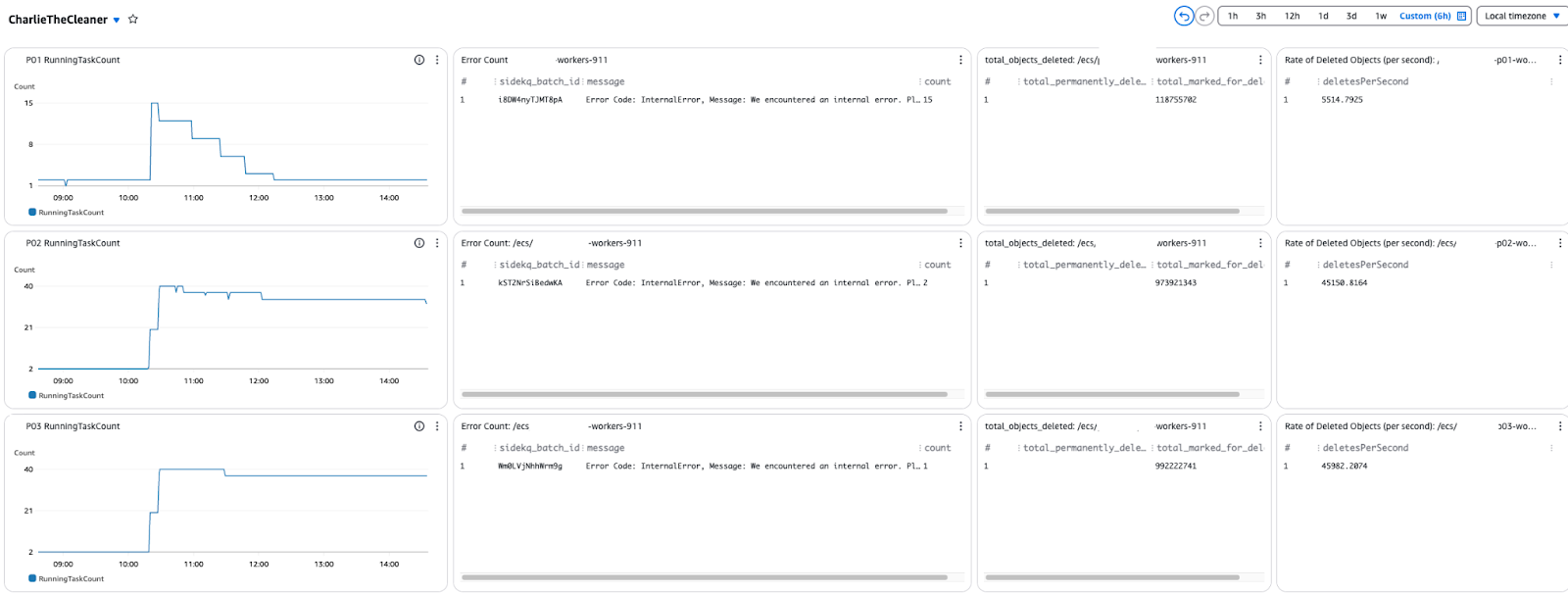
The dashboard included metrics on the ECS tasks and how they were scaling in/out, a quick view of any errors being encountered and metrics on the objects being deleted. We were especially interested in the overall rate of deletions we were seeing, so we could determine if we were on track for completing the project within our estimated timeframe.
Cloudwatch logs insights queries are powerful tools for showing metric data from simple log messages. This query was used to show the rate of deletions on the dashboard:
filter message like /objects from/ and level_index = 3| parse message /(?<action>Permanently deleted|Marked for delete) (?<deletedCount>\d+) objects from .* and platform_id: (?<platform_id>\d+)/| stats sum(deletedCount) / ((max(@timestamp) - min(@timestamp)) / 1000) as deletesPerSecondFinal results
When this project completed, here’s where we ended up:
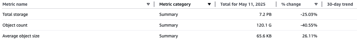
A total of 3.1 PB was removed with just over 120 billion objects removed (this was double our actual object count of 60 billion due to the additional delete markers placed).
Our S3 storage bill for our Shopify backups was reduced by 50%.
So how much did this cost us? Recall that our first approach was to use S3 batch tagging and rely on S3 lifecycle rules to remove the tagged content. This was estimated to cost around $300K.
Using the process described above, we incurred the following costs:
- AWS Glue to generate the object lists: $1500
- S3 Inventory reports: $800
- ECS Fargate Tasks: $260
This meant an overall cost of $2,560 or around $0.00000004 per object version.
Not bad when compared to $300K.
Conclusion
This project to remove duplicate data from S3 was driven by a desire to improve efficiency and optimize the product, not a mandate to cut costs. While storage costs were a major factor in the decision to pursue the work, the goal at Rewind is to use resources efficiently, not simply to conserve.
By continuously pushing ourselves to find the best solution, we didn’t just save money by addressing duplication—we streamlined processes to further long-term scalability. This project was about proactive improvement and exploring opportunities to make the product more robust and efficient for the future.
 Mandeep Khinda">